SCG is implemented in Python but can be accessed from R via the reticulate package. This page demonstrates how to load the pre-computed SCG results from the data application and work with them in R. We also show how to fit the model from scratch in R for users who prefer that workflow.
Setup
Note
Replace the path in use_python() with the path to your own Python installation that has scr installed. To find it, run which python or which python3 in your terminal. Please see reticulate for further guidance.
library(reticulate)library(ggplot2)library(dplyr)
Attaching package: 'dplyr'
The following objects are masked from 'package:stats':

    filter, lag
The following objects are masked from 'package:base':

    intersect, setdiff, setequal, union
When passing data from R to Python via reticulate, NumPy arrays are non-writable by default. This triggers a PyTorch warning during torch$as_tensor that can be safely ignored.
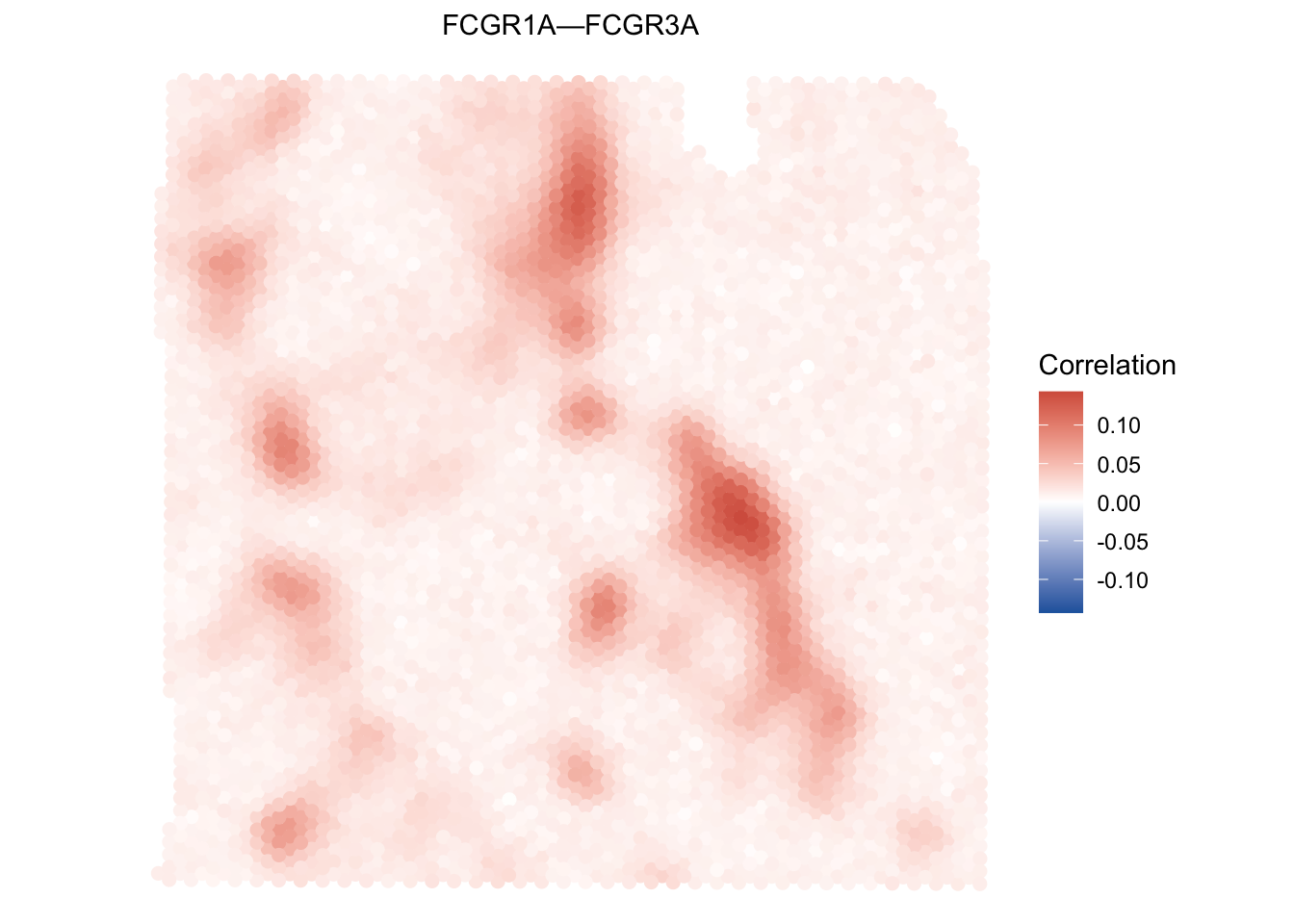
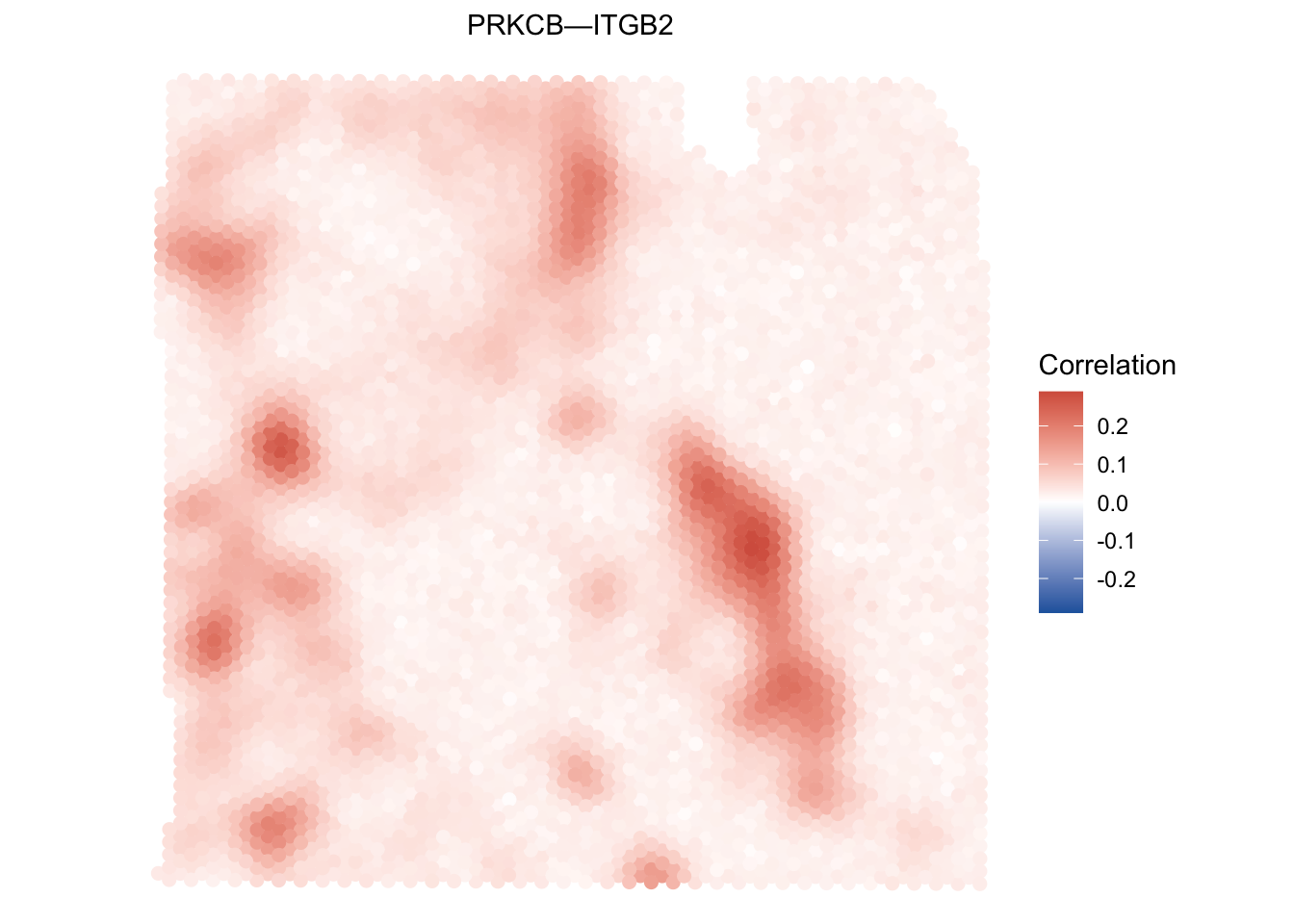
---title: "R Usage"---## OverviewSCG is implemented in Python but can be accessed from R via the [reticulate](https://rstudio.github.io/reticulate/) package. This page demonstrates how to load the pre-computed SCG results from the [data application](data-application.qmd) and work with them in R. We also show how to fit the model from scratch in R for users who prefer that workflow.## Setup::: {.callout-note}Replace the path in `use_python()` with the path to your own Python installation that has `scr` installed. To find it, run `which python` or `which python3` in your terminal. Please see [reticulate](https://rstudio.github.io/reticulate/) for further guidance. :::```{r}library(reticulate)library(ggplot2)library(dplyr)use_python("~/.pyenv/versions/3.11.14/bin/python")np <-import("numpy")```## Loading Pre-computed ResultsThe results from the data application are saved in `../results/` and can be loaded directly in R without re-fitting the model.### SCG Classifications```{r}results <-read.csv("../results/results.csv")spot_info <-read.csv("../data/spot_info.csv")gene_names <-read.csv("../data/gene_names.csv")scgs <- results[results$scg =="True", ]cat(nrow(scgs), "SCGs identified out of", nrow(results), "edges\n")```### Correlation Fields```{r}Corr_est <- np$load("../results/Corr_est.npy")dim(Corr_est)```## Visualizing Spatially Varying Edges```{r}boundary_colors <-c("T"="#7651A6", "N"="#2E7D6E", "I"="#C4952D")plot_corr_field <-function( Corr_est, spot_info, g, g_prime,gene_names =NULL) { field <- Corr_est[, g +1, g_prime +1] # convert 0-indexed to 1-indexed df <-data.frame(x = spot_info$x,y = spot_info$y,corr = field,region = spot_info$region ) vmax <-max(abs(df$corr)) g_label <-if (!is.null(gene_names)) { gene_names$gene[g +1] } else {as.character(g) } g_prime_label <-if (!is.null(gene_names)) { gene_names$gene[g_prime +1] } else {as.character(g_prime) }ggplot(df, aes(x = x, y = y, color = corr)) +geom_point(size =2.0) +scale_color_gradient2(low ="#2166ac",mid ="white",high ="#d6604d",midpoint =0,limits =c(-vmax, vmax),name ="Correlation" ) +coord_equal() +ggtitle(paste0(g_label, "—", g_prime_label)) +theme_void() +theme(legend.position ="right",plot.title =element_text(hjust =0.5, size =11) )}plot_corr_field( Corr_est, spot_info,g =2,g_prime =4,gene_names = gene_names)plot_corr_field( Corr_est, spot_info,g =39,g_prime =49,gene_names = gene_names)```## Fitting the Model from RUsers who wish to fit SCG from scratch in R can do so via `reticulate`. The workflow mirrors the Python data application exactly.```{r}#| eval: falsescr <-import("scr")torch <-import("torch")Y_np <-as.matrix(read.csv("../data/Y.csv"))Y_np <-t(Y_np)dims <-dim(Y_np)N <- dims[1]P <- dims[2]K <- L <-as.integer(round(2*log(P)))init <- scr$scr_init(Y = Y_np,L = L,K = K,a_delta =c(2.1, 3.1),b_delta =1.0,a0 =5.0,b0 =0.5,nu =5.0,spca_center =TRUE,spca_alpha =0.01,spca_ridge_alpha =0.01,device = scr$DEVICE,dtype = scr$DTYPE)kernel_hypers <- scr$pick_kernel_params(init = init,S =as.matrix(spot_info[, c("x", "y")]))K_np <- scr$rq_kernel(as.matrix(spot_info[, c("x", "y")]),v2 =1.0,rho =0.1* kernel_hypers$rho,alpha = kernel_hypers$alpha)fit <- scr$cavi( torch$as_tensor(Y_np, device = scr$DEVICE, dtype = scr$DTYPE), torch$as_tensor(K_np, device = scr$DEVICE, dtype = scr$DTYPE), init,max_iter =60L,verbose =FALSE)results <- scr$classify_edges(fit$params, M =500L, alpha =0.1)```::: {.callout-note}When passing data from R to Python via reticulate, NumPy arrays are non-writable by default. This triggers a PyTorch warning during `torch$as_tensor` that can be safely ignored.:::## Session Info```{r}sessionInfo()```